Using the Augmented Lagrangian function.
![]()
This tutorial demonstrates how to use the AugmentedLagrangian formulation to solve constrained optimization problems in Cooper. We illustrate its usage and advantages over the QuadraticPenalty formulation with a simple 2D example from [NW06].
%%capture
%pip install cooper-optim
import matplotlib.pyplot as plt
import torch

import cooper

DEVICE = torch.device("cuda" if torch.cuda.is_available() else "cpu")
Matplotlib is building the font cache; this may take a moment.
Problem Formulation
We consider the following constrained optimization problem (Problem 17.3 from Nocedal and Wright [NW06]) with a single equality constraint:
The unique solution is \(\boldsymbol{x}^* = (-1, -1)\).
The code below implements this constrained minimization problem.
class Problem2D(cooper.ConstrainedMinimizationProblem):
    def __init__(self, formulation_type):
        super().__init__()

        if not formulation_type.expects_multiplier:
            self.multiplier = None
        else:
            self.multiplier = cooper.multipliers.DenseMultiplier(num_constraints=1, device=DEVICE)

        if not formulation_type.expects_penalty_coefficient:
            self.penalty = None
        else:
            self.penalty = cooper.penalty_coefficients.DensePenaltyCoefficient(
                init=torch.tensor(0.0, device=DEVICE),
            )

        self.constraint = cooper.Constraint(
            constraint_type=cooper.ConstraintType.EQUALITY,
            formulation_type=formulation_type,
            multiplier=self.multiplier,
            penalty_coefficient=self.penalty,
        )

    def compute_cmp_state(self, x):
        objective = torch.sum(x)  # x1 + x2
        constraint = torch.sum(x**2) - 2  # x1^2 + x2^2 - 2 = 0

        constraint_state = cooper.ConstraintState(violation=constraint)

        return cooper.CMPState(loss=objective, observed_constraints={self.constraint: constraint_state})
The Augmented Lagrangian function associated with this problem is:
where \(\mu\) is the Lagrange multiplier associated with the equality constraint, and \(c\) is the penalty parameter.
We will also consider the Quadratic Penalty function associated with this problem:
Both of these formulations are instantiated in the following code block:
Solving the Problem
X_STAR = torch.tensor([-1.0, -1.0], device=DEVICE)


def train(problem, x, primal_lr, momentum, dual_lr, penalty_increment, n_steps):
    has_dual_variables = problem.multiplier is not None

    primal_optimizer = torch.optim.SGD([x], lr=primal_lr, momentum=momentum)

    if has_dual_variables:
        dual_optimizer = torch.optim.SGD(problem.dual_parameters(), lr=dual_lr, maximize=True)

        constrained_optimizer = cooper.optim.SimultaneousOptimizer(
            cmp=problem,
            primal_optimizers=primal_optimizer,
            dual_optimizers=dual_optimizer,
        )
    else:
        # Formulations without dual variables, such as the Quadratic Penalty
        # formulation, do not require a dual optimizer
        constrained_optimizer = cooper.optim.UnconstrainedOptimizer(
            cmp=problem,
            primal_optimizers=primal_optimizer,
        )

    # Increase the penalty coefficient by `increment` if the constraint is violate by more
    # than `violation_tolerance`
    penalty_scheduler = cooper.penalty_coefficients.AdditivePenaltyCoefficientUpdater(
        increment=penalty_increment,
        violation_tolerance=1e-3,
    )

    dist_2_x_star, multipliers, penalty_coefficients = [], [], []

    for _ in range(n_steps):
        roll_out = constrained_optimizer.roll(compute_cmp_state_kwargs={"x": x})

        # Update the penalty coefficient
        constraint_state = roll_out.cmp_state.observed_constraints[problem.constraint]
        penalty_scheduler.update_penalty_coefficient_(problem.constraint, constraint_state)

        multiplier_value = problem.multiplier.weight.item() if has_dual_variables else None
        penalty_coefficient_value = problem.constraint.penalty_coefficient().item()

        dist_2_x_star.append(torch.norm(x - X_STAR).item())
        multipliers.append(multiplier_value)
        penalty_coefficients.append(penalty_coefficient_value)

    return x, dist_2_x_star, multipliers, penalty_coefficients
primal_lr = 1e-2
momentum = 0.9
penalty_increment = 1e-2
n_steps = 5_000

# Only required for Augmented Lagrangian formulation
dual_lr = 1e-2

x_qp = torch.tensor([1.0, 1.0], device=DEVICE, requires_grad=True)
x_al = torch.tensor([1.0, 1.0], device=DEVICE, requires_grad=True)

QP_Problem = Problem2D(cooper.formulations.QuadraticPenalty)
AL_Problem = Problem2D(cooper.formulations.AugmentedLagrangian)

x_qp_final, dist_qp, qp_multipliers, qp_penalty_coefficients = train(
    QP_Problem, x_qp, primal_lr, momentum, dual_lr, penalty_increment, n_steps
)
x_al_final, dist_al, al_multipliers, al_penalty_coefficients = train(
    AL_Problem, x_al, primal_lr, momentum, dual_lr, penalty_increment, n_steps
)
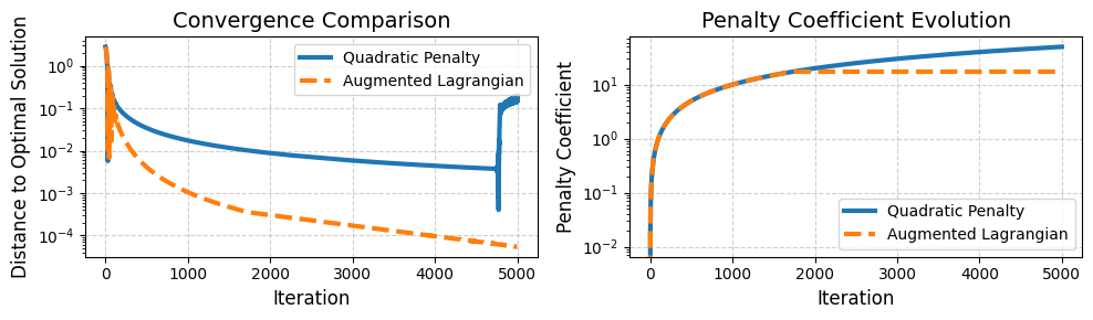
Results
The plot below illustrates that the Quadratic Penalty function requires a significantly larger penalty coefficient \(c\) to enforce feasibility compared to the Augmented Lagrangian function. This large penalty leads to numerical instability, preventing the algorithm’s convergence.
In contrast, the Augmented Lagrangian function achieves convergence with a finite penalty coefficient, avoiding these stability issues.
plt.figure(figsize=(10, 3))

# Plot distance to optimal solution
plt.subplot(1, 2, 1)
plt.plot(dist_qp, label="Quadratic Penalty", linewidth=3)
plt.plot(dist_al, label="Augmented Lagrangian", linewidth=3, linestyle="dashed")
plt.yscale("log")
plt.xlabel("Iteration", fontsize=12)
plt.ylabel("Distance to Optimal Solution", fontsize=12)
plt.title("Convergence Comparison", fontsize=14)
plt.legend()
plt.grid(True, linestyle="--", alpha=0.6)

# Plot penalty coefficients
plt.subplot(1, 2, 2)
plt.plot(qp_penalty_coefficients, label="Quadratic Penalty", linewidth=3)
plt.plot(al_penalty_coefficients, label="Augmented Lagrangian", linewidth=3, linestyle="dashed")
plt.yscale("log")
plt.xlabel("Iteration", fontsize=12)
plt.ylabel("Penalty Coefficient", fontsize=12)
plt.title("Penalty Coefficient Evolution", fontsize=14)
plt.legend()
plt.grid(True, linestyle="--", alpha=0.6)

plt.tight_layout()
plt.show()