Finding a spectrum-constrained linear transformation between two vectors.

Note

This example highlights the use of the flags contributes_to_primal_update and contributes_to_dual_update in the ConstraintState class. These flags are used to specify whether a constraint violation contributes to the primal or dual update. By default, both flags are set to True.

However, in this example, we update the primal parameters based on a surrogate constraint since the true constraint is expensive to compute, and difficult to differentiate. The true constraint is only computed every few iterations, and the multipliers are (infrequently) updated based on the true constraint.

Note that this update scheme is similar to the proxy-constraint approach. However, using proxy-constraints via the strict_violation argument in the ConstraintState class would still require the computation of the true constraint at every iteration. In this example, we avoid this by using the contributes_to_primal_update and contributes_to_dual_update flags, enabling the update of the primal and dual variables at different frequencies.

Consider the problem of finding the matrix \(X\) that transforms a vector \(y\) so as to minimize the mean squared error between \(Xy\) and another vector \(z\), under a constraint on the geometric mean of the singular values of \(X\). Formally,

\[ \min_{X} \,\, \Vert Xy - z \Vert_2^2 \,\, \text{ such that } \,\, \prod_{i=1}^r \sigma_i(X) = c^r \]

where \(X \in \mathbb{R}^{m \times n}\), \(y \in \mathbb{R}^m\), \(z \in \mathbb{R}^n\), \(r = \min\{m, n\}\), \(\sigma_i(X)\) denotes the \(i\)-th singular value of \(X\), and \(c\) is a constant.

We calculate the geometric mean of the singular values of \(X\) by first computing the singular value decomposition of \(X\). Note that the SVD decomposition is relatively expensive. However, the arithmetic mean of the squared singular values of \(X\) can be computed cheaply as it corresponds to the trace of \(X X^T\).

Therefore, we can use the arithmetic mean as a surrogate for the true constraint on the geometric mean of the singular values of X. While this choice of surrogate is not guaranteed to produce the same solution as the true constraint, the tutorial illustrates it is a good practical heuristic.

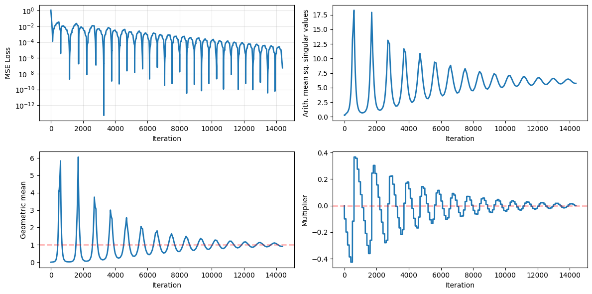
This example illustrates the ability to update the primal and dual variables at different frequencies. Here, we make use of the cheap surrogate constraint to update the primal variables at every iteration, while the multipliers are updated using the _true_ constraint which is only observed sporadically. Note how the multiplier value remains constant in-between measurements of the true constraint.

%%capture
%pip install cooper-optim

import random

import matplotlib.pyplot as plt
import numpy as np
import torch

import cooper

torch.manual_seed(0)
np.random.seed(0)
random.seed(0)

DEVICE = torch.device("cuda" if torch.cuda.is_available() else "cpu")


def create_vectors(dim_y: int, dim_z: int, seed: int = 0):
    """Create y and z such that Xy = z is true for a well-conditioned matrix X."""
    torch.manual_seed(seed=seed)

    # Create a random linear system with all singular values equal to 1.
    U, _, V = torch.linalg.svd(torch.randn(dim_z, dim_y))
    S = torch.eye(dim_z, dim_y)
    X_true = U @ S @ V.T

    y = torch.randn(dim_y, 1)
    y = y / torch.linalg.norm(y)

    z = X_true @ y
    z = z / torch.linalg.norm(z)

    y, z = y.to(DEVICE), z.to(DEVICE)

    return y, z


class MinNormWithSingularValueConstraints(cooper.ConstrainedMinimizationProblem):
    """Find a matrix X to minimize the error of a linear system, under a constraint on
    the geometric mean of the singular values of X.
    """

    def __init__(self, y: torch.Tensor, z: torch.Tensor, constraint_level: float = 1.0):
        super().__init__()

        self.y, self.z = y, z
        self.r = min(y.shape[0], z.shape[0])
        self.constraint_level = constraint_level

        # Creating a constraint with a single equality constraint
        constraint_type = cooper.ConstraintType.EQUALITY
        multiplier = cooper.multipliers.DenseMultiplier(num_constraints=1, device=DEVICE)
        self.sv_constraint = cooper.Constraint(
            constraint_type=constraint_type, formulation_type=cooper.formulations.Lagrangian, multiplier=multiplier
        )

    def loss_fn(self, X: torch.Tensor) -> torch.Tensor:
        """Compute the MSE loss function for a given X."""
        return torch.linalg.norm(X @ self.y - self.z).pow(2) / 2

    def compute_arithmetic_mean(self, X: torch.Tensor) -> torch.Tensor:
        """Compute the arithmetic mean of the squared singular values of X."""
        # We use the *arithmetic* mean of the squared singular values of X as a
        # surrogate for the true constraint given by the geometric mean of the singular
        # values of X.
        # Since the surrogate is only used to compute gradients, there is no need to set
        # a constraint level offset.
        # This is equivalent to computing the trace of X * X^T (and dividing by r)
        return torch.einsum("ij,ij->", X, X) / self.r

    @staticmethod
    @torch.no_grad()
    def compute_geometric_mean(X: torch.Tensor) -> torch.Tensor:
        return torch.linalg.svdvals(X).prod()

    def compute_surrogate_constraint(self, X: torch.Tensor) -> cooper.CMPState:
        """Compute the (differentiable) surrogate violation for the primal update."""
        # The `contributes_to_primal_update=True` and `contributes_to_dual_update=False`
        # flags indicate that the constraint is used to update the primal variables only.
        constraint_state = cooper.ConstraintState(
            violation=self.compute_arithmetic_mean(X),
            contributes_to_primal_update=True,
            contributes_to_dual_update=False,
        )

        return constraint_state

    def compute_true_constraint(self, X: torch.Tensor) -> cooper.CMPState:
        """Compute the non-differentiable constraint to update the multipliers."""
        # The `contributes_to_primal_update=False` and `contributes_to_dual_update=True`
        # flags indicate that the constraint is used to update the dual variables only.
        constraint_state = cooper.ConstraintState(
            violation=self.compute_geometric_mean(X) - self.constraint_level,
            contributes_to_primal_update=False,
            contributes_to_dual_update=True,
        )

        return constraint_state

    def compute_cmp_state(self, X: torch.Tensor, is_true_constraint: bool) -> cooper.CMPState:
        objective = self.loss_fn(X)

        if is_true_constraint:
            constraint_state = self.compute_true_constraint(X)
        else:
            constraint_state = self.compute_surrogate_constraint(X)

        return cooper.CMPState(loss=objective, observed_constraints={self.sv_constraint: constraint_state})


def run_experiment(dim_y, dim_z, constraint_level, max_iter, tolerance, freq_for_dual_update, primal_lr, dual_lr):
    y, z = create_vectors(dim_y=dim_y, dim_z=dim_z, seed=0)

    X = np.random.randn(dim_z, dim_y) / np.sqrt(dim_y * dim_z)

    # Creating X as a tensor from scratch for it to be a leaf tensor
    X = torch.tensor(X, requires_grad=True, device=DEVICE, dtype=torch.float32)

    cmp = MinNormWithSingularValueConstraints(y=y, z=z, constraint_level=constraint_level)
    primal_optimizer = torch.optim.SGD([X], lr=primal_lr)
    dual_optimizer = torch.optim.SGD(cmp.dual_parameters(), lr=dual_lr, maximize=True, foreach=False)
    cooper_optimizer = cooper.optim.AlternatingDualPrimalOptimizer(
        primal_optimizers=primal_optimizer, cmp=cmp, dual_optimizers=dual_optimizer
    )

    # Initial values of the loss, trace and geometric mean
    with torch.no_grad():
        state_history = {
            "loss": [cmp.loss_fn(X).item()],
            "arithmetic_mean": [cmp.compute_arithmetic_mean(X).item()],
            "geometric_mean": [cmp.compute_geometric_mean(X).item()],
            "multiplier_values": [cmp.sv_constraint.multiplier.weight.item()],
        }

    for it in range(max_iter):
        prev_X = X.clone().detach()

        cooper_optimizer.roll({"X": X, "is_true_constraint": (it % freq_for_dual_update) == 0})

        if prev_X.allclose(X, atol=tolerance):
            break

        with torch.no_grad():
            state_history["loss"].append(cmp.loss_fn(X).item())
            state_history["arithmetic_mean"].append(cmp.compute_arithmetic_mean(X).item())
            state_history["geometric_mean"].append(cmp.compute_geometric_mean(X).item())
            state_history["multiplier_values"].append(cmp.sv_constraint.multiplier.weight.item())

    return state_history


def plot_results(state_history, constraint_level):
    _, ax = plt.subplots(2, 2, figsize=(12, 6))

    ax[0, 0].plot(state_history["loss"])
    ax[0, 0].set_ylabel("MSE Loss")
    ax[0, 0].set_yscale("log")
    ax[0, 0].grid(True, which="both", alpha=0.3)

    ax[0, 1].plot(state_history["arithmetic_mean"])
    ax[0, 1].set_ylabel("Arith. mean sq. singular values")

    ax[1, 0].plot(state_history["geometric_mean"])
    ax[1, 0].set_ylabel("Geometric mean")
    # Horizontal line at desired `constraint_level`
    ax[1, 0].axhline(constraint_level, color="red", linestyle="--", alpha=0.3)

    ax[1, 1].plot(state_history["multiplier_values"])
    ax[1, 1].set_ylabel("Multiplier")
    ax[1, 1].axhline(0, color="red", linestyle="--", alpha=0.3)

    for ax_ in ax.flatten():
        ax_.set_xlabel("Iteration")
        for line in ax_.get_lines():
            line.set_linewidth(2)

    plt.tight_layout()

    plt.show()


dim_y, dim_z = 4, 4
constraint_level = 1.0 ** min(dim_y, dim_z)
primal_lr, dual_lr = 3e-2, 1e-1
freq_for_dual_update = 100
max_iter, tolerance = 50_000, 1e-6


state_history = run_experiment(
    dim_y=dim_y,
    dim_z=dim_z,
    constraint_level=constraint_level,
    max_iter=max_iter,
    tolerance=tolerance,
    freq_for_dual_update=freq_for_dual_update,
    primal_lr=primal_lr,
    dual_lr=dual_lr,
)
plot_results(state_history, constraint_level)