Learning a Directed Acyclic Graph (DAG) on data.
![]()
This tutorial considers the problem of learning a Directed Acyclic Graph (DAG) on data. This is a common problem in causal inference, where we are interested in learning the dependency relationships between variables. In this notebook, we will demonstrate how to learn a DAG on data using a QuadraticPenalty formulation in Cooper.
%%capture
%pip install cooper-optim
import math

import matplotlib.pyplot as plt
import networkx as nx
import numpy as np
import seaborn as sns
import torch

import cooper
Problem Formulation
Consider a \(d\)-dimensional random vector \({X_1, X_2, ..., X_d}\). Given \(n\) observations of the random vector \(X \in \mathbb{R}^{n \times d}\), we are interested in learning a DAG \(G = (V, E)\) whose edges represent the dependencies between the variables. We model the DAG via an adjacency matrix \(A \in \{0, 1\}^{d \times d}\), where \(A_{ij} = 1\) if there is an edge from \(X_i\) to \(X_j\) and \(A_{ij} = 0\) otherwise.
This problem can be formulated as the following optimization problem:
where \(\| \cdot \|_F\) is the Frobenius norm, \(r\) is a regularization parameter aimed at encougaing sparsity in the learned DAG, and the constraint ensures that the learned graph is acyclic.
Zheng et al. [ZARX18] show that the acyclicity constraint can be formulated as \(\text{tr}(e^{A}) = d\), where \(e^{A}\) is the matrix exponential of \(A\). This yields the following optimization problem:
Data Generation
The generative process we use is:
\(X_i \leftarrow \sum_{j \in \pi_i} X_j + \epsilon_i\)
where \(\pi_i\) is the set of parents of \(X_i\), and \(\epsilon_i \sim \mathcal{N}(0, \sigma^2)\) is Gaussian noise.
torch.manual_seed(1)
np.random.seed(1)


def generate_data(n: int, d: int, n_causes: int, noise_std: float, device: torch.device):
    """Generate data from a linear structural equation model with Gaussian noise.
    The

    Args:
        n: number of samples
        d: number of features
        n_causes: number of roots in the graph
        noise_std: standard deviation of the noise
        device: torch.device

    Returns:
        torch.Tensor: Data (X) of shape (n, d)
        torch.Tensor: Graph (A) of shape (d, d)
    """
    assert n_causes <= d

    # --------------------------------------------
    # Generate the adjacency matrix
    # --------------------------------------------

    # Rows are nodes, columns are parents
    A = torch.zeros(d, d, device=device)

    for i in range(n_causes, d):
        # For i=1, the only possible parent is 0
        parents = 0 if i == 1 else torch.randperm(i)[: np.random.randint(1, i)]

        A[i, parents] = 1

    assert torch.trace(torch.linalg.matrix_exp(A)).item() == d, "A is not a DAG"

    # --------------------------------------------
    # Sample data
    # --------------------------------------------

    noise = noise_std * torch.randn(n, d, device=device)
    X = torch.zeros(n, d, device=device)

    for i in range(d):
        parents = torch.nonzero(A[i]).flatten()
        X[:, i] = X[:, parents].sum(dim=1) + noise[:, i]

    # Improve conditioning
    X /= math.sqrt(d)

    return X, A
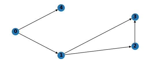
Now we generate the data and visualize the underlying DAG.
D = 5
N = 5_000
N_CAUSES = 1
NOISE_STD = 1e-2
DEVICE = torch.device("cuda" if torch.cuda.is_available() else "cpu")

# Generate data
X, A_TRUE = generate_data(N, D, N_CAUSES, NOISE_STD, DEVICE)
# Visualize the graph
G = nx.DiGraph()

G.add_nodes_from(range(D))
for i in range(D):
    for j in range(D):
        if A_TRUE[i, j] != 0:
            G.add_edge(j, i)

pos = nx.shell_layout(G)

plt.figure(figsize=(5, 2))
nx.draw(G, pos, with_labels=True, font_weight="bold")
plt.show()
Solving the Problem
We will use the QuadraticPenalty formulation to solve the problem. This leads to the following formulation of the constrained optimization problem:
where \(c\) is a penalty parameter. We will use a cooper.penalty_coefficients.AdditivePenaltyCoefficientUpdater to increase the penalty coefficient \(c\) whenever the constraint is violated beyond a tolerance.
ConstrainedMinimizationProblem
class DAGLearning(cooper.ConstrainedMinimizationProblem):
    def __init__(self, X: torch.Tensor, r: float):
        super().__init__()

        self.X = X
        self.n, self.d = X.shape
        self.r = r

        penalty_coefficient = cooper.penalty_coefficients.DensePenaltyCoefficient(
            init=torch.tensor(1.0, device=X.device),
        )
        self.constraint = cooper.Constraint(
            constraint_type=cooper.ConstraintType.EQUALITY,
            formulation_type=cooper.formulations.QuadraticPenalty,
            penalty_coefficient=penalty_coefficient,
        )

    def compute_cmp_state(self, A: torch.Tensor) -> cooper.CMPState:
        loss = torch.linalg.norm(self.X - self.X @ A.T, ord="fro") ** 2
        loss += self.r * torch.linalg.norm(A, ord=1)

        constraint_value = torch.trace(torch.linalg.matrix_exp(A)) - self.d
        constraint_state = cooper.ConstraintState(violation=constraint_value)

        return cooper.CMPState(loss=loss, observed_constraints={self.constraint: constraint_state})
Training
A = torch.nn.Parameter(torch.randn(D, D, device=DEVICE) / math.sqrt(D))

R = 1e-3
PRIMAL_LR = 1e-2
MOMENTUM = 0.9
N_STEPS = 2_000

cmp = DAGLearning(X, R)

primal_optimizer = torch.optim.SGD([A], lr=PRIMAL_LR, momentum=MOMENTUM)
constrained_optimizer = cooper.optim.UnconstrainedOptimizer(cmp=cmp, primal_optimizers=primal_optimizer)

# Increase the penalty coefficient by `increment` if the constraint is violate by more
# than `violation_tolerance`
penalty_scheduler = cooper.penalty_coefficients.AdditivePenaltyCoefficientUpdater(
    increment=1.0,
    violation_tolerance=1e-4,
)


steps, losses, violations, penalty_coefficients = [], [], [], []  # for plotting
for i in range(N_STEPS):
    roll_out = constrained_optimizer.roll(compute_cmp_state_kwargs={"A": A})

    A.data.fill_diagonal_(0)  # set the diagonal to zero to prevent self-loops
    A.data.clamp_(min=0, max=1)  # ensure that A is a valid adjacency matrix

    # Update the penalty coefficient
    constraint_state = roll_out.cmp_state.observed_constraints[cmp.constraint]
    penalty_scheduler.update_penalty_coefficient_(cmp.constraint, constraint_state)

    loss = roll_out.loss.item()
    violation = constraint_state.violation.item()
    penalty_coefficient_value = cmp.constraint.penalty_coefficient().item()

    if i % (N_STEPS // 100) == 0:
        steps.append(i)
        losses.append(loss)
        violations.append(violation)
        penalty_coefficients.append(penalty_coefficient_value)
Results
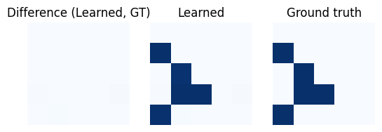
def plot_adjacency(adjacency, gt_adjacency):
"""Plot side by side: 1)the learned adjacency matrix, 2)the ground truth adj
matrix and 3)the difference of these matrices
:param np.ndarray adjacency: learned adjacency matrix
:param np.ndarray gt_adjacency: ground truth adjacency matrix
:param str exp_path: path where to save the image
:param str name: additional suffix to add to the image name
"""
plt.clf()
_, (ax1, ax2, ax3) = plt.subplots(ncols=3, nrows=1)
kwargs = {"vmin": 0, "vmax": 1, "cmap": "Blues", "xticklabels": False, "yticklabels": False}
sns.heatmap(adjacency, ax=ax2, cbar=False, **kwargs)
sns.heatmap(gt_adjacency, ax=ax3, cbar=False, **kwargs)
sns.heatmap(adjacency - gt_adjacency, ax=ax1, cbar=False, **kwargs)
ax1.set_title("Difference (Learned, GT)")
ax2.set_title("Learned")
ax3.set_title("Ground truth")
ax1.set_aspect("equal", adjustable="box")
ax2.set_aspect("equal", adjustable="box")
ax3.set_aspect("equal", adjustable="box")
plt.show()
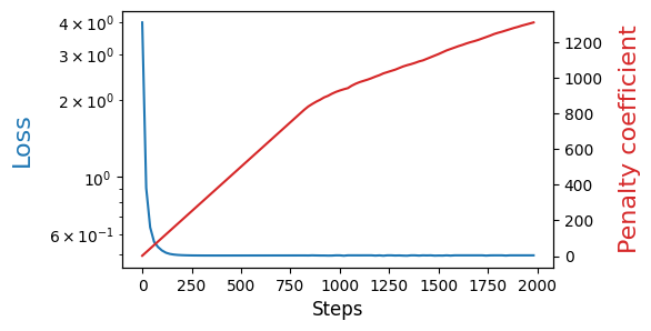
def plot_progress(steps, losses, penalty_coefficients):
_, ax1 = plt.subplots(figsize=(5, 3))
ax2 = ax1.twinx()
ax1.plot(steps, losses, "tab:blue")
ax2.plot(steps, penalty_coefficients, "tab:red")
ax1.set_yscale("log")
ax1.set_xlabel("Steps", fontsize=12)
ax1.set_ylabel("Loss", color="tab:blue", labelpad=10, fontsize=16)
ax2.set_ylabel("Penalty coefficient", color="tab:red", labelpad=10, fontsize=16)
plt.show()
Results
The following plot shows the loss and penalty coefficient as a function of the number of iterations. We can observe the following:
The loss decreases over time and eventually plateaus, as expected due to the noisy data generation process.
The penalty coefficient increases throughout training to enforce the acyclicity constraint. This increase is more pronounced early on because the initial DAG is not acyclic. Later, as the loss-driven updates to the DAG lead to constraint violations, the penalty coefficient continues to rise.
plot_progress(steps, losses, penalty_coefficients)
The next plot shows the adjacency matrix of the learned DAG, compared to the ground truth DAG. We can observe that we are able to recover the true DAG structure.
plot_adjacency(A.cpu().detach().numpy(), A_TRUE.cpu().detach().numpy())
<Figure size 640x480 with 0 Axes>